
Wednesday, 14 January, 2026г.


Где искать: по сайтам Запорожской области, статьи, видео ролики
пример: покупка автомобиля в Запорожье
How To Shade Every Other Row in Excel
 У вашего броузера проблема в совместимости с HTML5
This video shows you how to automatically apply shading to every nth row in a worksheet. You can apply the shading by using a simple conditional formatting formula.
1: Apply shading to alternate rows by using conditional formatting
One way to apply shading to alternate rows in your worksheet is by creating a conditional formatting rule. This rule uses a formula to determine whether a row is even or odd numbered, and then applies the shading accordingly. The formula is shown here:
=MOD(ROW(),2)=0
1. On the worksheet, do one of the following:
o To apply the shading to a specific range of cells, select the cells you want to format.
o To apply the shading to the entire worksheet, click the Select All button.
2. On the Home tab, in the Styles group, click the arrow next to Conditional Formatting, and then click New Rule.
3. In the New Formatting Rule dialog box, under Select a Rule Type, click Use a formula to determine which cells to format.
4. In the Format values where this formula is true box, enter =MOD(ROW(),2)=0, as shown in the following illustration.
Note: If you want to apply shading to alternate columns instead of alternate rows, enter =MOD(COLUMN(),2)=0 instead.
5. Click Format.
6. In the Format Cells dialog box, click the Fill tab.
7. Select the background or pattern color that you want to use for the shaded rows, and then click OK.
At this point, the color you just selected should appear in the Preview window in the New Formatting Rule dialog box.
8. To apply the formatting to the cells on your worksheet, click OK
Note: To view or edit the conditional formatting rule, on the Home tab, in the Styles group, click the arrow next to Conditional Formatting, and then click Manage Rules.
2: Apply shading to alternate rows by using an Excel table style
Another way to quickly add shading or banding to alternate rows is by applying a predefined Excel table style. This is useful when you want to format a specific range of cells, and you want the additional benefits that you get with a table, such the ability to quickly display total rows or header rows in which filter drop-down lists automatically appear.
By default, banding is applied to the rows in a table to make the data easier to read. The automatic banding continues if you add or delete rows in the table.
If you find you want the table style without the table functionality, you can convert the table to a regular range of data. If you do this, however, you won't get the automatic banding as you add more data to your range.
1. On the worksheet, select the range of cells that you want to format.
2. On the Home tab, in the Styles group, click Format as Table.
3. Under Light, Medium, or Dark, click the table style that you want to use.
4. In the Format as Table dialog box, click OK.
Notice that the Banded Rows check box is selected by default in the Table Style Options group.
If you want to apply shading to alternate columns instead of alternate rows, you can clear this check box and select Banded Columns instead.
5. If you want to convert the Excel table back to a regular range of cells, click anywhere in the table to display the tools necessary for converting the table back to a range of data.
6. On the Design tab, in the Tools group, click Convert to Range.
Tip: You can also right-click the table, click Table, and then click Convert to Range.
Music Credit
==========
Disfigure - Blank [NCS Release] https://youtu.be/p7ZsBPK656s
Похожие видео


![[Fix] Error formatting volume in Ubuntu and other Linux distributions](/images/mq/6/87/f_qppbVUczGq78.jpg)
Мой аккаунт